One Matrix, Two Cuts: Tensor Parallelism From Scratch
Tensor parallelism divides the computation of a single layer. The nonlinearity requires a column-parallel layer to come before a row-parallel layer. A full backward derivation shows that all weight-gradient computations remain local and only activation boundaries communicate. We verify a hand-written column-plus-row MLP against a single-GPU implementation, then measure TP sizes 2, 4 and 8 on PCIe.
1. From sharded storage to sharded computation
The previous four posts focused on storage sharding. ZeRO and FSDP divide parameters, gradients and optimizer states, but they gather each layer’s parameters before computation. The full matrix multiplication therefore still runs on every GPU. Tensor parallelism (TP) instead divides one multiplication, $Y = XW^\top$, across $N$ GPUs so that each performs roughly $1/N$ of the work.
A matrix can be divided along either dimension. We use the PyTorch layout $W \in \mathbb{R}^{d_{\text{out}} \times d_{\text{in}}}$ and activations $X \in \mathbb{R}^{bs \times d_{\text{in}}}$, with $Y = XW^\top$:
- Column cut (
ColumnParallelLinearin Megatron): split along $d_{\text{out}}$. Rank $k$ stores $W_k = W[k\frac{d_{\text{out}}}{N}:(k{+}1)\frac{d_{\text{out}}}{N},\,:]$, which contains complete rows. $X$ is replicated, so each rank computes its output block $Y_k = XW_k^\top$ without communication. Each rank holds only $1/N$ of the output features. - Row cut (
RowParallelLinear): split along $d_{\text{in}}$. Each rank must receive the corresponding input block $X_k$. It computes one partial output, and an all-reduce forms the complete result $Y = \sum_k X_k W_k^\top$.
Naming convention. Megatron names the cuts using $Y=XW$ with $W\in\mathbb{R}^{d_{\text{in}}\times d_{\text{out}}}$, so its column cut divides the output dimension. PyTorch stores linear weights as
[out, in], making the same partition a dim-0 row cut in memory. A reliable question is whether each fan-in row remains complete: it does underColumnParallelLinearand does not underRowParallelLinear. This distinction matters again in post #9.
2. Why the column cut comes before the row cut
The two cuts have matching interfaces. A column-parallel layer produces a feature-partitioned output, and a row-parallel layer expects a feature-partitioned input. Placing them next to each other therefore requires no communication between the two layers:
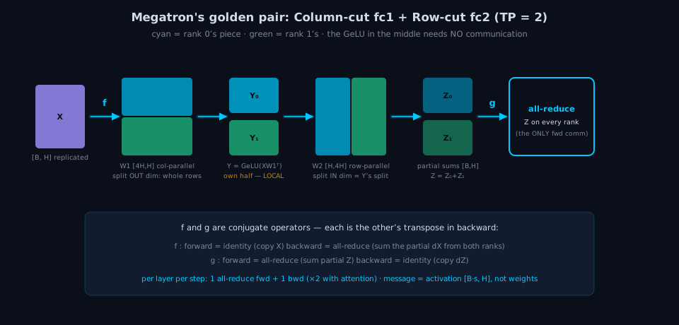
The full MLP dataflow (\(Z = \mathrm{GeLU}(XW_1^\top)W_2^\top\)):
\[X \xrightarrow{\ f\ } \underbrace{Y_k = \mathrm{GeLU}(XW_{1,k}^\top)}_{\text{Column cut, no comm}} \longrightarrow \underbrace{Z_k = Y_k W_{2,k}^\top}_{\text{Row cut, no comm}} \xrightarrow{\ g:\ \text{all-reduce}\ } Z = \textstyle\sum_k Z_k\]Each rank owns a complete block of pre-activation values, so it can apply GeLU locally. The MLP needs only one all-reduce, at the output of the row-parallel layer. Reversing the order does not work as well because GeLU is nonlinear:
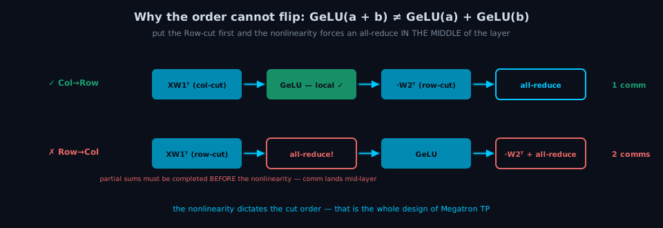
If fc1 is row-parallel, its output is only a partial sum and must be all-reduced before GeLU. A second collective is still needed after fc2, so the MLP would communicate twice instead of once. The position of the nonlinearity therefore determines the column-then-row order. Attention follows the same structure: QKV projections are column-parallel so that each rank owns complete heads, softmax runs locally within each head, and the output projection $W_O$ is row-parallel.
3. Backward pass: locating every communication
The backward pass shows exactly which tensors require communication. Write $\bar{A} \equiv \frac{\partial L}{\partial A}$. Given replicated $\bar{Z}$, the backward operation of $g$ is the identity:
(1) The row-parallel layer’s weight gradient is local:
\[\bar{W}_{2,k} = \bar{Z}^\top Y_k\]Every rank has $\bar{Z}$, and rank $k$ already stores $Y_k$. Both factors are local, so no communication is needed. The result $\bar{W}_{2,k}$ is the gradient of the weight shard owned by that rank and can also be stored and updated locally.
(2) The intermediate activation gradient is local:
\[\bar{Y}_k = \bar{Z}\, W_{2,k}, \qquad \bar{Y}^{\text{pre}}_k = \bar{Y}_k \odot \mathrm{GeLU}'(XW_{1,k}^\top)\]This uses only this rank’s \(W_{2,k}\) and this rank’s activations, so it is local.
(3) The column-parallel layer’s weight gradient is local:
\[\bar{W}_{1,k} = (\bar{Y}^{\text{pre}}_k)^\top X\]$X$ is replicated by the forward operation of $f$, and $\bar{Y}^{\text{pre}}_k$ is local. This multiplication therefore needs no communication.
(4) The input gradient requires an all-reduce:
\[\bar{X} = \sum_k \bar{Y}^{\text{pre}}_k W_{1,k}\]Each rank computes one term of this sum, so an all-reduce is required to form $\bar{X}$. This is the backward operation of $f$.
Together, the four equations give the following communication pattern:
All weight-gradient computations are local. Communication occurs only at activation boundaries: $g$ performs an all-reduce in forward, while $f$ performs one in backward. An MLP therefore uses one forward and one backward activation all-reduce. Attention uses the same pair, for a total of four activation all-reduces per transformer layer and training step.
Weight gradients remain local because both factors in each gradient multiplication are available on the rank that owns the corresponding weight shard. This follows from matching the partition layout to the dataflow. The same test applies to other parallel schemes: for each gradient formula, check whether every required factor is local.
4. Communication cost: TP moves activations, DP moves gradients
DP synchronizes gradients once per step, moving roughly $2\Psi$ bytes independent of batch size. TP communicates activations of shape $[bs \times h]$ four times per layer, so its volume grows with the number of tokens but not directly with parameter count. For $L$ layers and $\Psi \approx 12Lh^2$:
\[\frac{\text{TP comm per step}}{\text{DP comm per step}} = \frac{L \cdot 4 \cdot bsh}{\Psi} = \frac{4L \cdot bsh}{12Lh^2} = \frac{bs}{3h}\]The common $2\frac{N-1}{N}$ factor cancels when both use the same dtype. TP moves more data than DP once each rank processes more than $3h$ tokens, or 3840 tokens for GPT-2 Large, which is common during training. TP also communicates between layer computations through smaller, latency-sensitive collectives that are difficult to overlap. DP instead communicates large gradient buckets that can overlap with backward computation (post #2). This is why TP is usually kept within a node on the fastest available interconnect.
5. Experiment: numerical equivalence and PCIe scaling
A hand-written Column+Row MLP (~40 lines of core, ships with the post), GPT-2 Large geometry (h=1280, ff=5120, 4096 tokens), checked against a single GPU:
| TP | max forward error | max \(\bar{X}\) error |
|---|---|---|
| 2 | 3.8e-6 | 2.7e-12 |
| 4 | 3.8e-6 | 2.8e-12 |
| 8 | 3.3e-6 | 2.6e-12 |
The forward difference of about 1e-6 comes from fp32 summation order: all-reduce combines partial sums in a different order from the single-GPU matrix multiplication. The input-gradient difference is about 1e-12. TP changes the distribution of exact operations rather than introducing an algorithmic approximation.
Speed (one MLP forward, compute/communication decomposed):
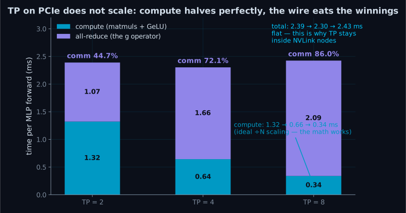
- Compute time decreases nearly in proportion to $N$: 1.32 → 0.64 → 0.34 ms.
- Communication time increases with $N$: the all-reduce message remains 21 MB ($[4096\times1280]$ in fp32), but the ring uses more steps and crosses more NUMA boundaries. Time rises from 1.07 to 1.66 to 2.09 ms. At TP=8, 21 MB in 2.09 ms corresponds to about 10 GB/s algbw, matching post #1’s all-reduce measurement.
- Total time remains almost unchanged: 2.39 → 2.30 → 2.43 ms, while communication grows from 45% to 72% to 86% of the total. On this machine without NVLink, the reduced compute time is offset by communication. With an interconnect about 25× faster, the communication estimate would fall by a similar factor and the TP=8 communication share would be about 20%.
6. Reading along in real source
Megatron-LM implements ColumnParallelLinear and RowParallelLinear in megatron/core/tensor_parallel/layers.py. The $f/g$ operators are in mappings.py: copy_to_tensor_model_parallel_region implements $f$, and reduce_from_tensor_model_parallel_region implements $g$.
nanotron provides TensorParallelColumnLinear with SplitConfig(split_dim=0) and TensorParallelRowLinear with split_dim=1 in src/nanotron/parallel/tensor_parallel/nn.py. The differentiable primitives in distributed_differentiable_primitives.py implement $f/g$ as autograd.Functions corresponding to the derivation in Section 3.
Our bench_tp.py reduces the implementation to one weight shard per rank and one all-reduce. The core communication pattern from Section 3 fits in about 40 lines.
7. Summary
- TP divides layer computation. A column-parallel layer produces the partitioned input required by a row-parallel layer, and the nonlinearity determines this order. No communication is needed between the pair.
- The backward derivation shows that all weight-gradient computations are local. Only activation boundaries communicate through $f$ in backward and $g$ in forward, giving four activation all-reduces per layer and step. The general test is whether every factor in each gradient multiplication is local.
- TP communication scales with activation size $bsh$, while DP communication scales with parameter count $\Psi$. Their volume ratio is $bs/3h$. Because TP collectives occur between layer computations and are difficult to overlap, TP is usually kept within a node.
- The implementation matches the single-GPU result up to floating-point summation order. On PCIe, compute time decreases with $N$ but total time remains flat because communication reaches 86% of the TP=8 runtime.
Next comes Sequence and Context Parallelism. TP divides weights and layer computation, but each rank still stores full $[b \times s \times h]$ activations at region boundaries. Sequence parallelism shards the LayerNorm and dropout activations left replicated by TP, while context parallelism addresses the larger memory and compute cost of long-context attention.
Environment: 8× RTX PRO 6000 Blackwell, PyTorch 2.9.1, NCCL 2.27.5. Reproduce: torchrun --standalone --nproc_per_node={2,4,8} bench_tp.py. Plotting and schematic code accompanies the series.
All benchmark scripts, schematic generators, plotting code and raw result CSVs for this post live in assets/blog/code/05-tensor-parallel.
Appendix: The Code That Ran
Every number in this post comes from the scripts below, embedded verbatim. Plotting and schematic code plus the raw result CSVs live in the folder linked above.
bench_tp.py
"""
TP experiment (part 05 of the Illustrated Distributed Training series): a hand-written
Megatron-style Column+Row parallel MLP.

Verifies two things:
  1. Correctness: an MLP with Column-cut fc1 + Row-cut fc2 matches the single-GPU
     forward output and backward gradients exactly (bit-for-bit in fp64, up to
     rounding in bf16). "Zero communication in the middle" is not an approximation.
  2. Cost: 1 all-reduce per layer in forward (the g operator), 1 in backward
     (the f operator). Measures the per-layer time breakdown (compute vs comm)
     for TP=2/4/8.

Usage:
  torchrun --standalone --nproc_per_node={2,4,8} bench_tp.py --out ../results/tp.csv
"""

import argparse
import csv
import os
import time

import torch
import torch.distributed as dist
import torch.nn.functional as F

H = 1280               # hidden size (GPT-2 Large scale)
FF = 4 * H             # 5120
MBS, SEQ = 4, 1024
WARMUP, STEPS = 20, 50


def main():
    ap = argparse.ArgumentParser()
    ap.add_argument("--out", default="../results/tp.csv")
    args = ap.parse_args()

    rank = int(os.environ["RANK"])
    world = int(os.environ["WORLD_SIZE"])
    local_rank = int(os.environ["LOCAL_RANK"])
    torch.cuda.set_device(local_rank)
    device = torch.device("cuda", local_rank)
    dist.init_process_group("nccl", device_id=device)

    torch.manual_seed(1337)  # same seed on every rank so weights match
    # full weights (fp32 so results can be reconciled exactly)
    W1 = torch.randn(FF, H, device=device) / H**0.5      # fc1 [out=FF, in=H]
    W2 = torch.randn(H, FF, device=device) / FF**0.5     # fc2 [out=H, in=FF]
    X = torch.randn(MBS * SEQ, H, device=device, requires_grad=True)

    # ---- single-GPU reference ----
    ref = F.gelu(X @ W1.t()) @ W2.t()
    ref_loss = ref.square().mean()
    ref_loss.backward()
    ref_grad = X.grad.clone()
    X.grad = None

    # ---- TP: Column-cut W1 (along out dim), Row-cut W2 (along in dim) ----
    shard = FF // world
    W1_k = W1[rank * shard:(rank + 1) * shard]            # [FF/N, H] whole rows
    W2_k = W2[:, rank * shard:(rank + 1) * shard]         # [H, FF/N] column slice

    Xtp = X.detach().clone().requires_grad_(True)
    # forward: f operator = identity (X already replicated), intermediate Y_k local, g operator = all-reduce
    Y_k = F.gelu(Xtp @ W1_k.t())                          # [B, FF/N] intermediate activation: zero comm
    Z_k = Y_k @ W2_k.t()                                  # [B, H] partial sum
    Z = Z_k.clone()
    dist.all_reduce(Z)                                    # g: the only forward comm
    loss = Z.square().mean()
    loss.backward()                                       # backward: dX is a partial sum
    gX = Xtp.grad.clone()
    dist.all_reduce(gX)                                   # f's backward: all-reduce dX

    fwd_err = (Z - ref).abs().max().item()
    grad_err = (gX - ref_grad).abs().max().item()

    # ---- timing: break down compute vs communication ----
    def timed(fn):
        s, e = torch.cuda.Event(True), torch.cuda.Event(True)
        dist.barrier(); torch.cuda.synchronize()
        s.record()
        for _ in range(STEPS):
            fn()
        e.record(); torch.cuda.synchronize()
        return s.elapsed_time(e) / STEPS

    def fwd_only():
        z = F.gelu(Xtp @ W1_k.t()) @ W2_k.t()
        return z

    def fwd_with_ar():
        z = F.gelu(Xtp @ W1_k.t()) @ W2_k.t()
        dist.all_reduce(z)
        return z

    for _ in range(WARMUP):
        fwd_with_ar()
    t_compute = timed(fwd_only)
    t_total = timed(fwd_with_ar)
    t_comm = t_total - t_compute

    if rank == 0:
        row = [world, fwd_err, grad_err, round(t_compute, 3), round(t_comm, 3),
               round(t_total, 3), round(t_comm / t_total * 100, 1)]
        newfile = not os.path.exists(args.out)
        os.makedirs(os.path.dirname(args.out) or ".", exist_ok=True)
        with open(args.out, "a", newline="") as f:
            w = csv.writer(f)
            if newfile:
                w.writerow(["tp", "fwd_max_err", "grad_max_err", "compute_ms", "comm_ms", "total_ms", "comm_pct"])
            w.writerow(row)
        print("ROW:", row, flush=True)
    dist.destroy_process_group()


if __name__ == "__main__":
    main()