The bf16 Bargain: A Numerics Ledger For Mixed Precision
Mixed-precision training uses low precision for frequently processed tensors and high precision for persistent state. This explains why computation can use bf16, why optimizer states remain fp32, and why fp16 often needs loss scaling. In a small experiment, all-bf16 training appears to work and even obtains lower validation loss, but an update audit shows that 87% of late-training parameter updates would round to zero. At a smaller learning rate, training without an fp32 master copy stalls.
1. Precision choices left unexplained
Earlier posts used mixed precision in several places without explaining the numerical reasons:
- Post #0 counts 2 bytes per parameter but 12 bytes per parameter for master parameters and Adam states. Why can computation use 2-byte values while optimizer state uses 4-byte values?
- Post #3 uses $K=12$ for fp32 master parameters and the fp32 Adam states $m$ and $v$. Why is a second parameter copy necessary?
- Post #4’s FSDP used
MixedPrecisionPolicy(param_dtype=bf16, reduce_dtype=fp32). Why does the reduction get its own dtype?
One principle connects these choices:
Individual multiplications can use lower precision, but long accumulations and persistent updates need higher precision.
2. Precision and range are different things
A floating-point format contains a sign, an exponent and a mantissa. Exponent bits determine range, while mantissa bits determine precision. fp16 and bf16 divide their 16 bits differently:
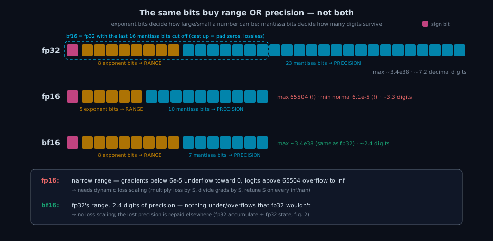
- fp16 has 5 exponent bits and 10 mantissa bits. It provides about 3.3 decimal digits of precision but a limited range, with a maximum of 65504 and a minimum normal value of 6.1e-5. Small gradients can enter the subnormal range or underflow to zero. In Section 4, 57% of measured gradients fall below 6.1e-5. Loss scaling multiplies the loss by a factor $S$ so that gradients remain representable, then divides them by $S$ before the optimizer update. Dynamic scaling adjusts $S$ when infinities or NaNs appear.
- bf16 has 8 exponent bits and 7 mantissa bits. It has the same exponent range as fp32, so values that are representable in fp32 do not underflow merely because they are cast to bf16. Loss scaling is therefore usually unnecessary. The trade-off is about 2.4 decimal digits of precision. Casting bf16 to fp32 only appends zeros and is exact. Casting fp32 to bf16 rounds away low mantissa bits.
On recent hardware, bf16 is often preferred to fp16 when its wider range is more useful. Its lower precision is managed by performing sensitive additions and accumulations in fp32.
3. The precision map of one training step
The dtype of each tensor follows its role in one training step:
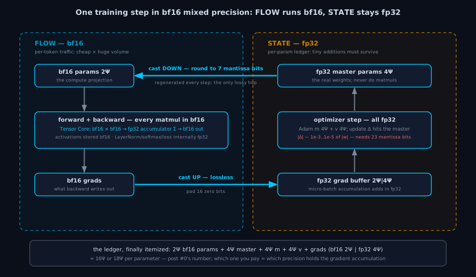
The left side of the figure contains flow tensors: activations and temporary gradients. Their volume scales with tokens, they are consumed quickly, and they can use bf16. The right side contains persistent state: master parameters, Adam moments and gradient-accumulation buffers. These values receive many small updates and remain in fp32. After backward, bf16 gradients are upcast exactly into fp32 buffers. After the optimizer step, fp32 master parameters are rounded to create the next bf16 compute copy.
Three mechanisms preserve fp32 accuracy where it matters:
Line 1: fp32 accumulation in Tensor Cores. A bf16 matrix multiplication forms bf16 products but accumulates them in fp32 before rounding the output. This matters because an inner product with $h=4096$ adds 4096 terms. In bf16, a small term can round away once the running sum becomes much larger. For example, adding 4096 copies of 0.01 sequentially gives 40.96 in fp32 but only 4.0 in bf16. After the bf16 sum reaches 4.0, an additional 0.01 is below half an ulp and no longer changes the result.
Line 2: fp32 gradient accumulation in software. Gradient accumulation also adds many small values. nanotron’s FP32GradientAccumulator in src/nanotron/optim/gradient_accumulator.py upcasts each microbatch’s bf16 gradient and adds it to a persistent fp32 buffer. This choice explains the difference between the 16Ψ and 18Ψ memory ledgers. Keeping gradients in bf16 saves 2Ψ bytes and reduces communication, while fp32 buffers use 2Ψ additional bytes and preserve small accumulated values. FSDP can keep parameter storage in lower precision while setting reduce_dtype=fp32 for reduction.
| Line 3: the fp32 master copy. The update $w \leftarrow w + \Delta$ adds a small change to a much larger stored value. In middle and late training, $ | \Delta | $ may be only $10^{-3}$ to $10^{-5}$ of $ | w | $. With 7 explicit mantissa bits, bf16 rounds sufficiently small updates back to the original value: |
| When an update falls below this threshold, storing the result in bf16 can leave the parameter unchanged. Starting from $w=1.0$ and adding $10^{-4}$ one thousand times produces 1.1 in fp32, while the bf16 value remains 1.0 when each update is rounded independently. Applying updates to an fp32 master parameter allows small changes to accumulate. fp32 has 23 explicit mantissa bits and can preserve updates down to roughly $ | w | \cdot 2^{-24}$. A new bf16 compute copy is then generated from the master after every step rather than updated in place. |
3.1 If fp32 is stored anyway, why not compute in it?
The fp32 master already exists, so one might use it directly for forward and backward and avoid the 2Ψ bf16 copy. That would make the dominant matrix multiplications much slower. The master parameter is touched once per step by an element-wise update, while the bf16 copy participates in almost every forward and backward matrix multiplication. For an $8192^3$ GEMM on one RTX PRO 6000, fp32 reaches 52.7 TFLOPS and bf16 reaches 262 TFLOPS, a 5.0× difference. TF32 reaches 133.4 TFLOPS and fp16 reaches 209.5 TFLOPS. The additional 2Ψ storage therefore keeps the small update in fp32 while running most computation, activation storage and communication in bf16.
4. Experiment: three precision schemes and an update audit
We train a character-level GPT with 6 layers, width 384 and about 10M parameters on Tiny Shakespeare for 6000 steps on one GPU. The learning rate follows a cosine schedule from 1e-3 to 1e-4. All three schemes use the same initialization and batch sequence. Only their precision policy changes:
| scheme | params | compute | Adam state | master copy |
|---|---|---|---|---|
fp32 | fp32 | fp32 | fp32 | not needed (parameters are already fp32) |
mixed | fp32 | autocast bf16 | fp32 | ✓ (the fp32 params) |
bf16 | bf16 | bf16 | bf16 | ✗ (naive “everything bf16”) |
| fp32 | mixed | bf16 (no master) | |
|---|---|---|---|
| step time | 36.5 ms | 10.2 ms (3.6×) | 8.9 ms |
| peak memory | 2.51 GiB | 1.64 GiB (−35%) | 1.27 GiB |
| train loss @6000 (EMA) | 0.078 | 0.079 | 0.079 |
| val loss @6000 | 4.26 | 4.24 | 3.51 |
The results require three observations:
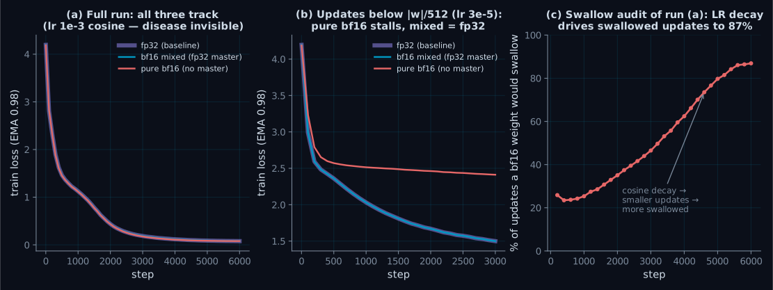
- Mixed precision closely matches fp32 while running 3.6× faster and using 35% less peak memory. Their final EMA training losses are 0.079 and 0.078, and their curves nearly overlap in panel (a).
- Naive all-bf16 training does not fail in this small run. Its training loss follows the other schemes, and its final validation loss is lower, at 3.51 versus 4.24 for mixed precision. The 10M-parameter model begins overfitting the 1.1M-character dataset near step 1300. bf16 rounding noise appears to regularize the model and delay overfitting. This result does not show whether the optimizer can preserve small useful updates later in training.
- Panel (c) measures the fraction of updates that would be lost to bf16 rounding. Every 200 steps in the mixed run, we take the fp32 update $\Delta$ and simulate applying it to each bf16 parameter. The fraction for which $(w_{\rm bf16}+\Delta)$ rounds back to $w_{\rm bf16}$ rises from about 25% at the initial learning rate to 87% after cosine decay. This has little visible effect once the small task is already fitted, but it can matter when useful updates become small before training is complete.
| Panel (b) isolates this regime by training the same model from scratch with a constant learning rate of 3e-5. Many updates are then near or below the $ | w | /512$ threshold. Mixed precision and fp32 both reach a loss of 1.50. Pure bf16 falls to 2.57 during the first 500 steps, when gradients are larger, but then improves only to 2.41 by step 3000. With an fp32 master, small updates accumulate until they change the projected bf16 copy. Without a master, each update can round away independently before accumulation occurs. |
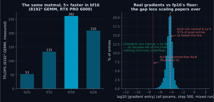
The left panel reports the 5× GEMM throughput difference discussed in Section 3.1. The right panel shows the distribution of parameter gradients at step 500. Fifty-seven percent are below fp16’s minimum normal value of 6.1e-5, where values become subnormal and lose precision. About 0.05% underflow to zero. Multiplying the loss by 1024 shifts this distribution about three orders of magnitude upward before the gradients are unscaled. bf16 and fp32 have a minimum normal value near 1.2e-38, far below the measured range.
Boundary of the experiment. The constant small-learning-rate run isolates the rounding mechanism rather than following a typical training schedule. In larger and longer runs, parameter updates often become small relative to parameter values during normal middle and late training. Our all-bf16 scheme also stores Adam’s $m$ and $v$ states in bf16. The second moment $v$ accumulates squared gradients and can be even more sensitive, which is why production systems usually keep optimizer states in fp32.
5. Reading along in real source
PyTorch autocast: torch/amp uses operation-specific dtype rules. Matrix multiplication and convolution can run in bf16, while operations such as softmax, LayerNorm and losses may remain fp32. PyTorch inserts the required casts at operation boundaries.
FSDP2: MixedPrecisionPolicy(param_dtype=torch.bfloat16, reduce_dtype=torch.float32), used in post #4. Sharded params (state) stay in fp32, all-gathered compute copies (flow) run in bf16, and the reduce-scatter happens in fp32.
nanotron: FP32GradientAccumulator in src/nanotron/optim/gradient_accumulator.py is the textbook implementation of defense line 2.
Megatron-LM: Float16OptimizerWithFloat16Params in megatron/core/optimizer/optimizer.py does the main_params (fp32 master) / model_params (bf16) double bookkeeping, plus --accumulate-allreduce-grads-in-fp32.
DeepSpeed ZeRO: the optimizer state sharded by stage 1 includes fp32 master parameters. ZeRO-1 therefore shards $(4+4+4)\Psi$ bytes of master parameters and Adam moments across $N$ ranks, while the 2Ψ bf16 compute copy remains replicated.
6. Summary, and closing the series
- Precision and range are separate properties. fp16 provides more mantissa bits but a narrower exponent range, so small gradients may require loss scaling. bf16 uses fp32’s exponent width and usually avoids loss scaling, but retains only about 2.4 decimal digits of precision.
- Flow tensors use bf16, while persistent state uses fp32. Activations and temporary gradients account for most per-token volume. Master parameters, optimizer moments and accumulation buffers need fp32 for repeated small additions. Hardware fp32 accumulation, exact bf16-to-fp32 casts and per-step projection connect the two.
-
Updates below the stated $ w /512$ threshold can round to no parameter change in bf16. The audit reaches 87% after learning-rate decay. The small default run hides this effect because rounding noise also reduces overfitting, but the constant-small-LR run separates the mechanisms: the no-master model stalls at 2.41 while mixed precision reaches 1.50. - The 16Ψ and 18Ψ ledgers from post #0 consist of 2Ψ bf16 parameters, 4Ψ fp32 master parameters, 4Ψ each for Adam’s $m$ and $v$, and either 2Ψ or 4Ψ for gradients depending on accumulation precision.
This closes the series. The nine posts use four recurring tools: communication volume from post #1, the $\Psi$ memory ledger, schedule geometry and numerical precision. Together they provide a way to evaluate a new parallel training method by identifying what it stores, what it communicates, when it waits and where it loses numerical information.
Environment: 8× RTX PRO 6000 Blackwell (1 used), PyTorch 2.9.1, CUDA 12.8. Reproduce: python train_precision.py (main comparison + swallow audit + gradient histogram), python train_precision.py --steps 3000 --warmup 0 --lr 3e-5 --min-lr 3e-5 --tag _lowlr (small-LR mechanism isolation), and python bench_gemm.py (GEMM throughput). Plotting and schematic code accompanies the series.
All benchmark scripts, schematic generators, plotting code and raw result CSVs for this post live in assets/blog/code/08-mixed-precision.
Appendix: The Code That Ran
Every number in this post comes from the scripts below, embedded verbatim. Plotting and schematic code plus the raw result CSVs live in the folder linked above.
train_precision.py
"""
Three-precision comparison training (part 08 of the Illustrated Distributed Training
series): same model, same data, same random seeds, only the precision scheme changes.
Measures the claim "mixed precision converges like fp32 at bf16 speed, pure bf16
trains badly".

Three schemes:
  fp32    params and compute all fp32 (baseline)
  mixed   fp32 params (i.e. the master copy) + autocast bf16 compute, the de facto bf16 mixed precision
  bf16    params, momentum, and compute all bf16, no fp32 master copy, the naive "drop the master copy" scheme

Two extra ledgers (both inside the mixed run, where fp32 params are a trustworthy reference):
  1. swallow fraction: every 200 steps, actually round this step's fp32 update delta
     to bf16 and count how many params satisfy (w+delta).bf16 == w.bf16. If params
     were bf16, these updates would be swallowed whole.
  2. gradient histogram: log10|g| distribution over all parameter gradients at step 500,
     compared against the representable lower bounds of fp16/bf16.

Model: char-level GPT (6 layers, width 384, ~10M params, self-contained definition,
SDPA attention so all three dtypes can run, whereas the repo's model.py hard-depends
on flash-attn which only accepts fp16/bf16), tiny-shakespeare, single GPU.
Usage: python train_precision.py --outdir ../results
"""

import argparse
import csv
import math
import os

import numpy as np
import torch
import torch.nn as nn
import torch.nn.functional as F


class Block(nn.Module):
    def __init__(self, n_embd, n_head):
        super().__init__()
        self.n_head = n_head
        self.ln1 = nn.LayerNorm(n_embd, bias=False)
        self.attn = nn.Linear(n_embd, 3 * n_embd, bias=False)
        self.proj = nn.Linear(n_embd, n_embd, bias=False)
        self.ln2 = nn.LayerNorm(n_embd, bias=False)
        self.fc = nn.Linear(n_embd, 4 * n_embd, bias=False)
        self.fc_proj = nn.Linear(4 * n_embd, n_embd, bias=False)

    def forward(self, x):
        B, T, C = x.shape
        q, k, v = self.attn(self.ln1(x)).split(C, dim=2)
        q, k, v = (t.view(B, T, self.n_head, C // self.n_head).transpose(1, 2) for t in (q, k, v))
        y = F.scaled_dot_product_attention(q, k, v, is_causal=True)
        x = x + self.proj(y.transpose(1, 2).reshape(B, T, C))
        x = x + self.fc_proj(F.gelu(self.fc(self.ln2(x))))
        return x


class GPT(nn.Module):
    def __init__(self, vocab, block, n_layer=6, n_head=6, n_embd=384):
        super().__init__()
        self.tok = nn.Embedding(vocab, n_embd)
        self.pos = nn.Embedding(block, n_embd)
        self.blocks = nn.ModuleList([Block(n_embd, n_head) for _ in range(n_layer)])
        self.ln_f = nn.LayerNorm(n_embd, bias=False)
        self.head = nn.Linear(n_embd, vocab, bias=False)
        self.head.weight = self.tok.weight  # weight tying
        self.apply(lambda m: torch.nn.init.normal_(m.weight, 0.0, 0.02)
                   if isinstance(m, (nn.Linear, nn.Embedding)) else None)

    def forward(self, idx, targets):
        x = self.tok(idx) + self.pos(torch.arange(idx.shape[1], device=idx.device))
        for b in self.blocks:
            x = b(x)
        logits = self.head(self.ln_f(x))
        loss = F.cross_entropy(logits.view(-1, logits.size(-1)), targets.view(-1))
        return logits, loss

BLOCK, BATCH = 256, 64
MAX_ITERS, WARMUP_ITERS = 6000, 100
LR, MIN_LR = 1e-3, 1e-4
EVAL_INTERVAL, EVAL_ITERS = 100, 20
SWALLOW_INTERVAL = 200
GRADHIST_STEP = 500
DEVICE = torch.device("cuda", 0)


def load_data():
    text = open(os.path.join(os.path.dirname(__file__), "input.txt")).read()
    chars = sorted(set(text))
    stoi = {c: i for i, c in enumerate(chars)}
    data = np.array([stoi[c] for c in text], dtype=np.uint16)
    n = int(0.9 * len(data))
    return data[:n], data[n:], len(chars)


def get_batch(data, gen):
    ix = torch.randint(len(data) - BLOCK - 1, (BATCH,), generator=gen)
    x = torch.stack([torch.from_numpy(data[i:i + BLOCK].astype(np.int64)) for i in ix])
    y = torch.stack([torch.from_numpy(data[i + 1:i + 1 + BLOCK].astype(np.int64)) for i in ix])
    return x.pin_memory().to(DEVICE, non_blocking=True), y.pin_memory().to(DEVICE, non_blocking=True)


def lr_at(it):
    if it < WARMUP_ITERS:
        return LR * (it + 1) / WARMUP_ITERS
    t = (it - WARMUP_ITERS) / (MAX_ITERS - WARMUP_ITERS)
    return MIN_LR + 0.5 * (LR - MIN_LR) * (1 + math.cos(math.pi * t))


@torch.no_grad()
def evaluate(model, val, autocast_ctx):
    model.eval()
    gen = torch.Generator().manual_seed(4242)  # all three runs use the same validation batches
    losses = []
    for _ in range(EVAL_ITERS):
        x, y = get_batch(val, gen)
        with autocast_ctx():
            _, loss = model(x, y)
        losses.append(loss.float().item())
    model.train()
    return sum(losses) / len(losses)


def run(scheme, train, val, vocab, outdir, tag=""):
    torch.manual_seed(1337)
    torch.cuda.manual_seed_all(1337)
    torch.cuda.empty_cache()
    torch.cuda.reset_peak_memory_stats()

    model = GPT(vocab, BLOCK).to(DEVICE)
    if scheme == "bf16":
        model = model.bfloat16()  # params are bf16, and Adam momentum follows the param dtype so it is bf16 too

    if scheme == "mixed":
        def autocast_ctx():
            return torch.autocast("cuda", dtype=torch.bfloat16)
    else:
        from contextlib import nullcontext
        autocast_ctx = nullcontext

    opt = torch.optim.AdamW(model.parameters(), lr=LR, betas=(0.9, 0.95),
                            weight_decay=0.1, eps=1e-8)
    gen = torch.Generator().manual_seed(1337)  # all three runs consume the same stream of training batches

    curve, swallow_rows, hist_rows = [], [], []
    step_times = []
    train_ema = None  # EMA of train loss (0.98), shows stagnation better than val once overfitting starts
    ev0 = torch.cuda.Event(enable_timing=True)
    ev1 = torch.cuda.Event(enable_timing=True)

    for it in range(MAX_ITERS):
        for g in opt.param_groups:
            g["lr"] = lr_at(it)
        x, y = get_batch(train, gen)

        ev0.record()
        with autocast_ctx():
            _, loss = model(x, y)
        loss.backward()

        # ---- swallow ledger (mixed: params are fp32, simulate how many updates bf16 params would swallow) ----
        do_swallow = scheme == "mixed" and (it + 1) % SWALLOW_INTERVAL == 0
        if do_swallow:
            prev = [p.detach().clone() for p in model.parameters()]
        # ---- gradient histogram (mixed, step 500) ----
        if scheme == "mixed" and it + 1 == GRADHIST_STEP:
            g_all = torch.cat([p.grad.detach().float().abs().flatten()
                               for p in model.parameters() if p.grad is not None])
            g_all = g_all[g_all > 0]
            logg = torch.log10(g_all)
            cnt = torch.histc(logg, bins=56, min=-12, max=2)
            edges = torch.linspace(-12, 2, 57)
            for lo, c in zip(edges[:-1].tolist(), cnt.tolist()):
                hist_rows.append([round(lo, 2), int(c)])

        opt.step()
        opt.zero_grad(set_to_none=True)
        ev1.record()
        torch.cuda.synchronize()
        if it >= 20 and not do_swallow:
            step_times.append(ev0.elapsed_time(ev1))
        li = loss.float().item()
        train_ema = li if train_ema is None else 0.98 * train_ema + 0.02 * li

        if do_swallow:
            tot, sw = 0, 0
            with torch.no_grad():
                for p, w0 in zip(model.parameters(), prev):
                    delta = p.detach() - w0
                    w0b = w0.bfloat16()
                    swallowed = (w0b.float() + delta).bfloat16() == w0b
                    sw += swallowed.sum().item()
                    tot += p.numel()
            swallow_rows.append([it + 1, round(sw / tot, 4)])
            print(f"  [swallow] step {it+1}: {sw/tot:.1%}", flush=True)

        if (it + 1) % EVAL_INTERVAL == 0 or it == 0:
            vl = evaluate(model, val, autocast_ctx)
            curve.append([it + 1, round(vl, 4), round(train_ema, 4)])
            print(f"[{scheme}] step {it+1}: val {vl:.4f} train_ema {train_ema:.4f}", flush=True)

    peak_gib = torch.cuda.max_memory_allocated() / 2**30
    step_ms = sum(step_times) / len(step_times)
    final_val = curve[-1][1]

    with open(os.path.join(outdir, f"curve_{scheme}{tag}.csv"), "w", newline="") as f:
        w = csv.writer(f); w.writerow(["step", "val_loss", "train_ema"]); w.writerows(curve)
    if swallow_rows:
        with open(os.path.join(outdir, f"swallow{tag}.csv"), "w", newline="") as f:
            w = csv.writer(f); w.writerow(["step", "swallow_frac"]); w.writerows(swallow_rows)
    if hist_rows:
        with open(os.path.join(outdir, "gradhist.csv"), "w", newline="") as f:
            w = csv.writer(f); w.writerow(["log10_bin_lo", "count"]); w.writerows(hist_rows)
    return [scheme, round(step_ms, 2), round(peak_gib, 3), final_val]


def main():
    global MAX_ITERS, WARMUP_ITERS, LR, MIN_LR, GRADHIST_STEP
    ap = argparse.ArgumentParser()
    ap.add_argument("--outdir", default="../results")
    ap.add_argument("--steps", type=int, default=MAX_ITERS)
    ap.add_argument("--warmup", type=int, default=WARMUP_ITERS)
    ap.add_argument("--lr", type=float, default=LR)
    ap.add_argument("--min-lr", type=float, default=MIN_LR)
    ap.add_argument("--tag", default="")  # use --tag _lowlr for the small-LR mechanism experiment
    args = ap.parse_args()
    MAX_ITERS, WARMUP_ITERS, LR, MIN_LR = args.steps, args.warmup, args.lr, args.min_lr
    if args.tag:
        GRADHIST_STEP = -1  # record the histogram only in the main experiment
    os.makedirs(args.outdir, exist_ok=True)

    train, val, vocab = load_data()
    print(f"vocab {vocab}, train {len(train)/1e6:.2f}M chars", flush=True)

    summary = []
    for scheme in ["fp32", "mixed", "bf16"]:
        print(f"=== {scheme} ===", flush=True)
        summary.append(run(scheme, train, val, vocab, args.outdir, args.tag))
    with open(os.path.join(args.outdir, f"summary{args.tag}.csv"), "w", newline="") as f:
        w = csv.writer(f)
        w.writerow(["scheme", "step_ms", "peak_mem_gib", "final_val_loss"])
        w.writerows(summary)
    for row in summary:
        print("SUMMARY:", row)


if __name__ == "__main__":
    main()
bench_gemm.py
"""
GEMM throughput vs precision (part 08 of the Illustrated Distributed Training series):
the same 8192^3 matmul, only the dtype changes, measured in TFLOPS. This is the
ledger behind "why 99% of the compute should run in low precision".

fp32   classic fp32 (TF32 off)
tf32   fp32 inputs, Tensor Core TF32 path (mantissa truncated to 10 bits)
bf16   bf16 inputs, fp32 accumulation (Tensor Core)
fp16   fp16 inputs, fp32 accumulation (Tensor Core)

Usage: python bench_gemm.py --out ../results/gemm.csv
"""

import argparse
import csv
import os

import torch

N = 8192
WARMUP, STEPS = 10, 50
DEVICE = torch.device("cuda", 0)


def bench(dtype, allow_tf32):
    torch.backends.cuda.matmul.allow_tf32 = allow_tf32
    a = torch.randn(N, N, device=DEVICE, dtype=dtype)
    b = torch.randn(N, N, device=DEVICE, dtype=dtype)
    for _ in range(WARMUP):
        a @ b
    ev0 = torch.cuda.Event(enable_timing=True)
    ev1 = torch.cuda.Event(enable_timing=True)
    ev0.record()
    for _ in range(STEPS):
        a @ b
    ev1.record()
    torch.cuda.synchronize()
    ms = ev0.elapsed_time(ev1) / STEPS
    tflops = 2 * N**3 / (ms / 1e3) / 1e12
    return ms, tflops


def main():
    ap = argparse.ArgumentParser()
    ap.add_argument("--out", default="../results/gemm.csv")
    args = ap.parse_args()

    rows = []
    for name, dtype, tf32 in [("fp32", torch.float32, False),
                              ("tf32", torch.float32, True),
                              ("bf16", torch.bfloat16, False),
                              ("fp16", torch.float16, False)]:
        ms, tflops = bench(dtype, tf32)
        rows.append([name, round(ms, 3), round(tflops, 1)])
        print(f"{name}: {ms:.2f} ms, {tflops:.1f} TFLOPS", flush=True)

    os.makedirs(os.path.dirname(args.out) or ".", exist_ok=True)
    with open(args.out, "w", newline="") as f:
        w = csv.writer(f)
        w.writerow(["dtype", "ms", "tflops"])
        w.writerows(rows)


if __name__ == "__main__":
    main()