The Geometry Of Pipeline Bubbles
Pipeline bubbles come from dependencies between stages and microbatches. This post derives the fraction $(p-1)/(m+p-1)$, explains how 1F1B reduces activation memory without changing the bubble, and identifies the costs that the formula omits. A roughly 60-line GPipe implementation on 4 GPUs matches the formula within 0.9% at $m{=}1$.
1. Pipeline stages perform different parts of the model
In DP, TP, SP and CP, every GPU performs the same type of operation on different data or tensor slices. Pipeline parallelism (PP) instead assigns different layers to different GPUs. The model is divided by depth into $p$ stages, and point-to-point sends and receives transfer activations and gradients across stage boundaries.
PP has relatively low communication volume. At each boundary and for each microbatch, it sends one $[b_{mb} \times h]$ activation forward and the corresponding gradient backward. These transfers are point-to-point rather than collective and do not scale with parameter count. PP is therefore less sensitive to interconnect bandwidth than TP and is often placed across nodes.
The trade-off is idle time between dependent stages. Stage 1 cannot begin a microbatch until stage 0 produces its activations, and stage 0 cannot begin its backward work until gradients return from later stages. This unavoidable idle region is the pipeline bubble.
2. Bubble geometry: a derivation by counting grid cells
Divide time into slots, where one slot represents one microbatch running through one stage. GPipe splits a batch into $m$ microbatches, executes all forward passes, and then executes all backward passes:
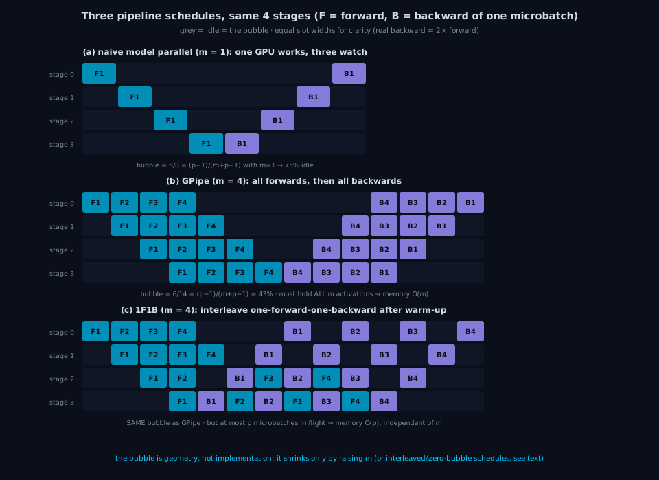
In panel (b), with $p{=}4$ and $m{=}4$, the first microbatch needs $p$ slots to reach the final stage. Each later slot completes one additional microbatch, so forward spans $m+p-1$ slots. Backward has the same length. Each stage performs $2m$ working slots during a total span of $2(m+p-1)$ slots:
\[\boxed{\ \text{bubble fraction} \;=\; \frac{2(m+p-1) - 2m}{2(m+p-1)} \;=\; \frac{p-1}{m+p-1}\ }\]The formula gives three direct conclusions:
- $m{=}1$ reduces to naive model parallelism in panel (a). The bubble fraction is $(p-1)/p$, which means 75% idle time on 4 stages and 87.5% on 8 stages.
- Increasing $m$ amortizes pipeline fill and drain. Setting $m=4p$ gives a bubble near 19%, while $m=8p$ gives about 10%. Gradient accumulation already divides an optimizer step into multiple microbatches, so it naturally supplies the required $m$ (post #2).
- The idealized bubble fraction depends on schedule shape rather than kernel or link speed. Faster operations shorten every slot but do not change the fraction of empty slots. Changing that fraction requires a different schedule.
3. 1F1B: the same bubble with lower activation memory
GPipe retains activations for all $m$ microbatches until backward begins, so activation memory is O(m). This conflicts with the need for a large $m$. 1F1B, or one-forward-one-backward in PipeDream-Flush, changes the order of operations. After a warm-up of $p-s$ forward passes for stage $s$, each stage alternates between one forward and one ready backward operation, as shown in panel (c):
- The total schedule length is the same as GPipe, so the bubble fraction is unchanged. Panels (b) and (c) contain the same number of idle cells.
- At most $p$ microbatches are active at once, so activation memory is O(p) rather than O(m). Increasing $m$ no longer increases the number of stored activation sets.
More advanced schedules modify the same dependency grid. Interleaved 1F1B assigns multiple non-adjacent model chunks to each GPU and reduces the bubble by the number of virtual stages. Zero-bubble schedules such as ZB-H1 separate input-gradient and weight-gradient computation to fill idle slots. DualPipe, used by DeepSeek-V3, runs pipelines in both directions.
4. Experiment: measuring GPipe across microbatch counts
The included GPipe implementation uses 4 stages, each with 6 Linear+GeLU layers of width 4096. The total batch remains fixed at 8192 rows while $m$ varies from 1 to 32. isend/recv connects adjacent stages, and backward sends ins[i].grad to the previous stage.
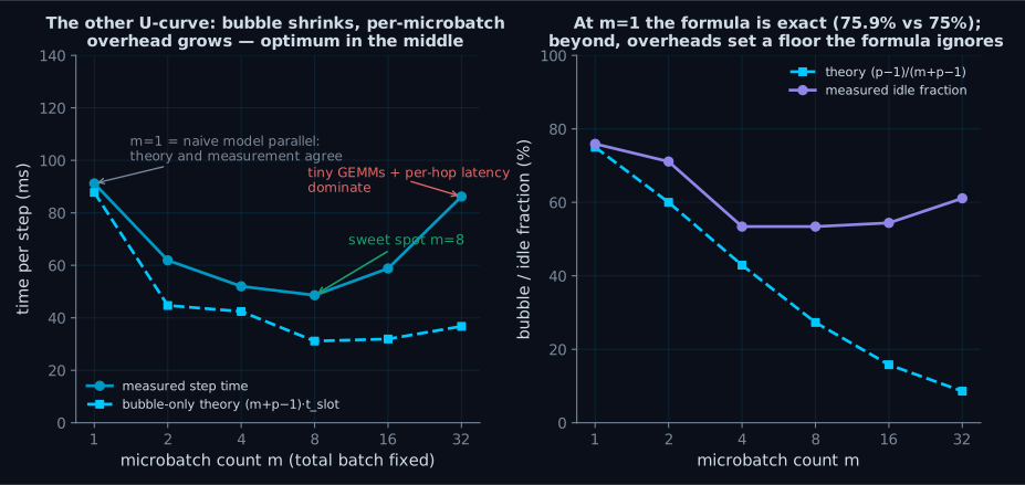
| m | 1 | 2 | 4 | 8 | 16 | 32 |
|---|---|---|---|---|---|---|
| step (ms) | 91.2 | 61.9 | 52.0 | 48.6 | 58.8 | 86.2 |
| bubble, theory | 75% | 60% | 43% | 27% | 16% | 9% |
| idle, measured | 75.9% | 71% | 53% | 53% | 54% | 61% |
The measurements show three effects:
- At $m{=}1$, measured idle time is 75.9% compared with the theoretical 75%. The difference is 0.9 percentage points.
- As $m$ grows, measured idle time stops improving near 53% and then increases. The geometric formula assumes fixed-cost slots, but every microbatch adds point-to-point latency and kernel-launch overhead. Smaller matrix multiplications are also less efficient. Reducing each microbatch from 8192 to 256 rows keeps total FLOPs constant but raises $m \cdot t_{\text{slot}}$ from 21.9 to 33.6 ms, a roughly 35% loss in execution efficiency.
- Bubble reduction favors a large $m$, while per-microbatch efficiency favors a smaller $m$. Their balance produces the best result at $m{=}8$ in this experiment. Production systems increase $m$ while also using interleaved or zero-bubble schedules, rather than relying only on ever smaller microbatches.
Boundary of the experiment. The implementation uses GPipe with equal slot times and no overlap between communication and computation. Production systems overlap sends and receives with compute, backward often takes about twice as long as forward, and stages may be imbalanced, especially around embeddings and the language-model head. These factors change the optimal $m$ but not the trade-off between pipeline bubbles and per-microbatch overhead.
5. Reading along in real source
PyTorch provides ScheduleGPipe and Schedule1F1B in torch.distributed.pipelining. Their operation order corresponds directly to panels (b) and (c).
nanotron: AllForwardAllBackwardPipelineEngine (= GPipe) and OneForwardOneBackwardPipelineEngine (= 1F1B) in src/nanotron/parallel/pipeline_parallel/engine.py, with p2p in p2p.py.
Megatron-LM keeps the schedules in megatron/core/pipeline_parallel/schedules.py, including interleaved 1F1B.
DeepSpeed compiles schedules into instruction streams such as LoadMicroBatch, ForwardPass and SendActivation in deepspeed/runtime/pipe/schedule.py.
6. Summary
- PP communicates point-to-point boundary activations rather than parameter-sized collectives, but stage dependencies create idle time. Under equal slot times, the bubble fraction is $\frac{p-1}{m+p-1}$.
- With $m{=}1$, the idle fraction is $(p-1)/p$. The experiment matches this value within 0.9 percentage points. Increasing the number of microbatches amortizes pipeline fill and drain, which makes gradient accumulation a natural fit for PP.
- 1F1B keeps the same idealized bubble fraction while reducing activation memory from O(m) to O(p). It changes peak memory without changing the schedule length.
- Point-to-point latency, kernel launches and small-GEMM inefficiency create an optimal finite $m$. The geometric bubble formula captures dependency idle time but not these per-microbatch costs.
Next comes mixed precision and the numerical role of bf16 and fp32. Earlier posts used FSDP’s MixedPrecisionPolicy, fp32 master parameters in ZeRO and fp32 gradient reductions without explaining their numerical purpose. The next post explains why computation can use bf16 while optimizer state remains fp32, and why fp16 requires loss scaling while bf16 usually does not.
Environment: 8× RTX PRO 6000 Blackwell (4 used), PyTorch 2.9.1, NCCL 2.27.5. Reproduce: torchrun --standalone --nproc_per_node=4 bench_gpipe.py. Plotting and schematic code accompanies the series, and the 1F1B slots are derived from dependency constraints, so verify them.
All benchmark scripts, schematic generators, plotting code and raw result CSVs for this post live in assets/blog/code/07-pipeline-parallel.
Appendix: The Code That Ran
Every number in this post comes from the scripts below, embedded verbatim. Plotting and schematic code plus the raw result CSVs live in the folder linked above.
bench_gpipe.py
"""
Hand-written GPipe (part 07 of the Illustrated Distributed Training series): measure
the bubble fraction vs microbatch count.

p stages (one per GPU), total batch fixed, sweep microbatch count m from 1 to 32:
  theory: T(m) = (m + p - 1) * t_slot   (t_slot = single-stage time for one microbatch)
  bubble fraction = (p-1) / (m + p - 1)
m=1 is naive model parallelism (only 1 GPU working at a time). Larger m thins the bubble.

Usage:
  torchrun --standalone --nproc_per_node=4 bench_gpipe.py --out ../results/gpipe.csv
"""

import argparse
import csv
import os
import time

import torch
import torch.distributed as dist
import torch.nn as nn

D = 4096                # hidden width
LAYERS_PER_STAGE = 6    # layers per stage
TOTAL_ROWS = 8192       # total batch (rows), fixed
M_LIST = [1, 2, 4, 8, 16, 32]
WARMUP, STEPS = 3, 10


class Stage(nn.Module):
    def __init__(self):
        super().__init__()
        self.layers = nn.Sequential(*[
            nn.Sequential(nn.Linear(D, D, bias=False), nn.GELU())
            for _ in range(LAYERS_PER_STAGE)])

    def forward(self, x):
        return self.layers(x)


def main():
    ap = argparse.ArgumentParser()
    ap.add_argument("--out", default="../results/gpipe.csv")
    args = ap.parse_args()

    rank = int(os.environ["RANK"])
    world = int(os.environ["WORLD_SIZE"])       # = p
    local_rank = int(os.environ["LOCAL_RANK"])
    torch.cuda.set_device(local_rank)
    device = torch.device("cuda", local_rank)
    dist.init_process_group("nccl", device_id=device)
    p = world

    torch.manual_seed(1337 + rank)
    stage = Stage().to(device).bfloat16()
    opt = torch.optim.SGD(stage.parameters(), lr=1e-4)  # cheap step: we only measure schedule geometry

    def gpipe_step(m):
        rows = TOTAL_ROWS // m
        ins, outs, reqs = [], [], []
        # ---- forward: m microbatches flow through one after another ----
        for i in range(m):
            if rank == 0:
                x = torch.randn(rows, D, device=device, dtype=torch.bfloat16)
                x.requires_grad_(True)
            else:
                x = torch.empty(rows, D, device=device, dtype=torch.bfloat16)
                dist.recv(x, src=rank - 1)
                x.requires_grad_(True)
            out = stage(x)
            if rank < p - 1:
                reqs.append(dist.isend(out.detach(), dst=rank + 1))
            ins.append(x)
            outs.append(out)
        for r_ in reqs:
            r_.wait()
        # ---- backward: reverse order ----
        for i in reversed(range(m)):
            if rank == p - 1:
                loss = outs[i].float().square().mean() / m
                loss.backward()
            else:
                g = torch.empty_like(outs[i])
                dist.recv(g, src=rank + 1)
                outs[i].backward(g)
            if rank > 0:
                dist.send(ins[i].grad, dst=rank - 1)
        opt.step()
        opt.zero_grad(set_to_none=True)

    # ---- t_slot: fwd+bwd time of one microbatch on this stage (no communication) ----
    def slot_time(m):
        rows = TOTAL_ROWS // m
        x = torch.randn(rows, D, device=device, dtype=torch.bfloat16, requires_grad=True)
        torch.cuda.synchronize()
        t0 = time.perf_counter()
        for _ in range(STEPS):
            out = stage(x)
            out.float().square().mean().backward()
            x.grad = None
            stage.zero_grad(set_to_none=True)
        torch.cuda.synchronize()
        return (time.perf_counter() - t0) / STEPS * 1e3

    rows_out = []
    for m in M_LIST:
        for _ in range(WARMUP):
            gpipe_step(m)
        dist.barrier(); torch.cuda.synchronize()
        t0 = time.perf_counter()
        for _ in range(STEPS):
            gpipe_step(m)
        torch.cuda.synchronize()
        step_ms = (time.perf_counter() - t0) / STEPS * 1e3
        t_slot = slot_time(m)
        if rank == 0:
            bubble_theory = (p - 1) / (m + p - 1)
            t_ideal = m * t_slot          # ideal time with no bubble and no communication
            bubble_meas = 1 - t_ideal / step_ms
            rows_out.append([p, m, round(t_slot, 2), round(step_ms, 1),
                             round(bubble_theory, 3), round(bubble_meas, 3)])
            print("ROW:", rows_out[-1], flush=True)

    if rank == 0:
        os.makedirs(os.path.dirname(args.out) or ".", exist_ok=True)
        with open(args.out, "w", newline="") as f:
            w = csv.writer(f)
            w.writerow(["p", "m", "slot_ms", "step_ms", "bubble_theory", "bubble_measured"])
            w.writerows(rows_out)
    dist.destroy_process_group()


if __name__ == "__main__":
    main()