The Price Of All-Reduce
Distributed training is built from six collective communication primitives. This post defines them, derives the exact per-GPU communication volume $2\frac{N-1}{N}S$ for ring all-reduce, and measures their performance on our 8-GPU machine. The benchmark and plotting code are included with the post.
DDP, ZeRO, FSDP, TP and PP all combine the same six collective communication primitives in different ways. The rest of this series uses these operations to compare communication costs. We therefore begin with three questions: What does each primitive do? How many bytes does each GPU send? How long does the operation take on real hardware?
We use the following accounting convention throughout the series:
Communication volume is the total number of bytes one GPU sends during one operation. Here, $S$ is the total size of the logical tensor in bytes, and $N$ is the process-group size. We count sends only. Modern interconnects such as NVLink, PCIe and InfiniBand are full-duplex, and balanced collectives send and receive the same amount of data per GPU.
1. The six primitives, one figure
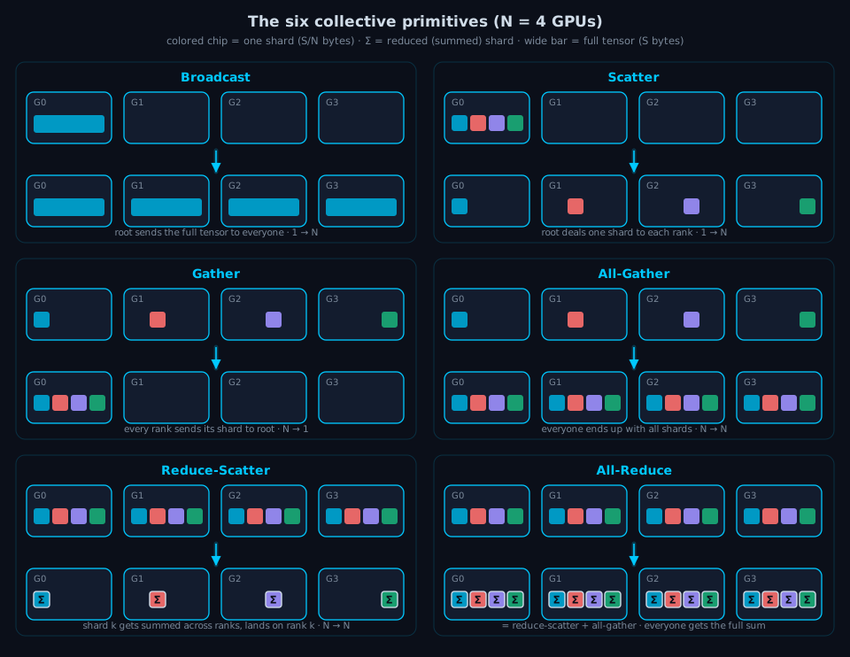
The table summarizes the data flow, per-GPU send volume and training role of each primitive:
| Primitive | Semantics (\(N\) GPUs) | Per-GPU send volume | Role in training |
|---|---|---|---|
| broadcast | root’s full tensor copied to everyone | ≈ \(S\) per GPU (ring implementation) | weight sync at init |
| scatter | root cuts the tensor into \(N\) shards, shard \(k\) → rank \(k\) | root sends \(\frac{N-1}{N}S\), others 0 | distributing data/state |
| gather | inverse scatter: all shards collected at root | each sends \(\frac{S}{N}\) | collecting results |
| all-gather | each rank starts with one shard. Afterwards, everyone holds the full concatenation | \(\frac{N-1}{N}S\) | ZeRO-3/FSDP parameter fetch |
| reduce-scatter | each rank starts with a full tensor. Shard \(k\) of the sum lands on rank \(k\) | \(\frac{N-1}{N}S\) | ZeRO gradient sync |
| all-reduce | element-wise sum of everyone’s tensor, result on everyone | \(2\frac{N-1}{N}S\) | DDP gradient sync |
Two properties are especially useful:
- all-reduce = reduce-scatter + all-gather. Reduce-scatter first places the sum of shard $k$ on rank $k$. All-gather then distributes every completed shard to every rank. Their communication volumes add up to $\frac{N-1}{N}S + \frac{N-1}{N}S = 2\frac{N-1}{N}S$. NCCL implements all-reduce using this two-phase structure. ZeRO uses the same identity but performs local computation between the two phases (post #3).
- The
all-primitives have no root, so every rank has the same role. Broadcast, scatter and gather use a root rank, whose link can become the bottleneck. Section 4 shows this difference in the measurements.
In PyTorch they map one-to-one onto torch.distributed:
import torch.distributed as dist

dist.broadcast(t, src=0)                    # root's t overwrites everyone's
dist.scatter(out, chunks, src=0)            # root sends chunks[k] to rank k
dist.gather(t, outs, dst=0)                 # everyone's t collected at root
dist.all_gather_into_tensor(out, t)         # out = concat of everyone's t, for everyone
dist.reduce_scatter_tensor(out, t)          # out = this rank's shard of the group sum
dist.all_reduce(t)                          # t = element-wise group sum, in place
Collectives are synchronization points. Every rank in the group must call the same operation with matching shapes and dtypes. If one rank does not participate, the others wait indefinitely.
2. Ring all-reduce: two phases, \(N-1\) steps each
A centralized implementation would send every tensor to rank 0, sum them there, and broadcast the result. The root would receive and send $(N-1)S$ bytes, so its traffic would grow linearly with $N$ while many other links remained underused. In contrast, each GPU fundamentally needs to send about $S$ bytes so that its data enters the sum and receive about $S$ bytes so that it obtains the result. An efficient algorithm should approach this lower bound while using all links in parallel.
Ring all-reduce approaches this bound. It arranges the $N$ GPUs in a logical ring, splits the tensor into $N$ shards, runs $N-1$ reduce-scatter steps, and then runs $N-1$ all-gather steps:
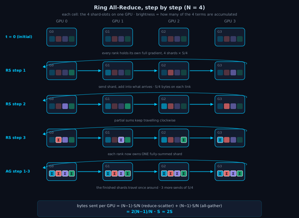
The two phases work as follows:
- Phase 1, reduce-scatter (RS steps 1–3): at each step, every GPU sends one shard, receives one shard, and adds the received values to its local partial sum. Within a single step, the four links each carry a different shard — the figure colors and numbers each arc to match the shard it carries, and rings the destination slot with that same color plus a
+when it has just been added into. A worked example above the panels spells out one hop as an actual addition: own share + arriving shard = one more term summed. After $N-1$ steps, each GPU owns one fully reduced shard (Σ). - Phase 2, all-gather (AG steps 1–3): the completed shards circulate around the ring without further arithmetic until every GPU has all Σ shards.
- At every step, each GPU sends to its successor and receives from its predecessor at the same time. This uses both directions of the full-duplex link. Send and receive volumes are equal, which is why we report only the send volume.
Per-GPU communication volume. Each GPU sends one $\frac{S}{N}$-byte shard in each of $2(N-1)$ steps:
\[\boxed{\;\text{per-GPU send} \;=\; 2(N-1)\cdot\frac{S}{N} \;=\; 2\,\frac{N-1}{N}\,S \;\xrightarrow{\;N\to\infty\;}\; 2S\;}\]The bandwidth volume per GPU is bounded by $2S$, which is essential for scalable data parallelism. However, the number of communication steps still grows with $N$. The time model separates these bandwidth and latency costs:
\[T_{\text{ring}} \;\approx\; 2(N-1)\left(\frac{S/N}{B} + \alpha\right) \;=\; \underbrace{2\,\frac{N-1}{N}\cdot\frac{S}{B}}_{\text{bandwidth term, } \approx 2S/B} \;+\; \underbrace{2(N-1)\,\alpha}_{\text{latency term, linear in } N}\]where \(B\) is the one-directional link bandwidth and \(\alpha\) the fixed per-step overhead (kernel launch + one hop). Two regimes follow:
- Large $S$: the bandwidth term dominates, so $T \approx 2S/B$ and depends only weakly on $N$.
- Small $S$: the latency term dominates, so $T \approx 2(N-1)\alpha$. Increasing the tensor size has little effect, while increasing $N$ raises the cost linearly.
The boundary between the regimes is directly visible in the measurements (§4.3), and it is the entire reason DDP buckets small gradients into big ones (post #2).
3. Understanding algbw and busbw
Collective benchmarks commonly report two bandwidth metrics. We follow the nccl-tests convention in every plot below:
- Algorithm bandwidth $\text{algbw} = S/t$ measures how quickly the user’s logical tensor is processed. Because different primitives move different amounts of data for the same $S$, algbw is not directly comparable across primitives.
- Bus bandwidth $\text{busbw} = \text{algbw} \times \text{correction}$ adjusts for the communication pattern’s actual traffic. It provides a more comparable view of link utilization across primitives and machines.
| Primitive | Correction factor | Source |
|---|---|---|
| all-reduce | \(2\frac{N-1}{N}\) | the derivation above |
| all-gather / reduce-scatter | \(\frac{N-1}{N}\) | single-phase ring |
| broadcast | \(1\) | each GPU relays ≈ \(S\) |
| scatter / gather | \(\frac{N-1}{N}\) | root-side traffic |
At the same tensor size $S$, all-reduce moves about twice as much data as all-gather. Its algbw should therefore be about half as large. Section 4 tests this prediction.
4. Experiments: six primitives on eight GPUs
Setup (the series’ standard environment):
| Hardware | 8× NVIDIA RTX PRO 6000 Blackwell (96 GB), pure PCIe, no NVLink |
| Topology | GPUs paired under PCIe switches (0-1/2-3/4-5/6-7), dual NUMA, UPI across sockets |
| Software | PyTorch 2.9.1 + cu128, NCCL 2.27.5, bf16 tensors |
| Method | CUDA-event timing, ≥5 warm-up iterations, mean of 10–50 runs. Launched with torchrun --standalone |
| Sweep | \(S\) from 4 KiB to 1 GiB, \(N \in \{2, 4, 8\}\) |
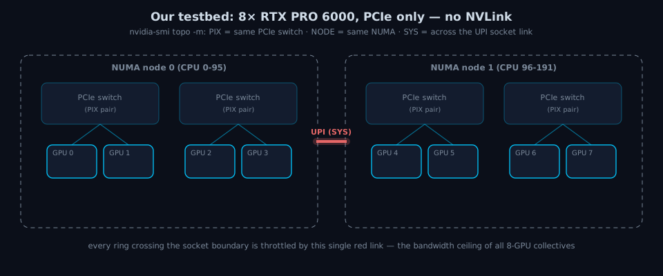
This machine has no NVLink. Its PCIe topology makes communication bottlenecks easier to observe.
4.1 Bus bandwidth of the six primitives
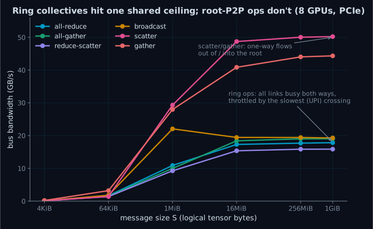
The measurements show three main results:
- The four ring-based collectives (all-reduce, all-gather, reduce-scatter and broadcast) converge to the same ~16–19 GB/s busbw plateau. Although the algorithms move different logical volumes, normalizing by their traffic factors reveals the same bottleneck link. On this machine, the ring crosses the UPI connection between CPU sockets, and the effective one-directional bandwidth is about 18 GB/s.
- Scatter and gather reach 44–50 GB/s because they use rooted, one-way point-to-point transfers rather than a ring. This exposes the practical one-directional bandwidth of a PCIe Gen5 x16 link. The same hardware delivers about 2.5× different effective bandwidth under a different communication pattern, so performance depends on both the algorithm and the topology.
- The measurements confirm AR = RS + AG. At $S = 1$ GiB, $t_{\text{AR}} = 105.3$ ms, while $t_{\text{RS}} + t_{\text{AG}} = 59.2 + 49.3 = 108.5$ ms, a difference of 3%. The algbw prediction from Section 3 also holds: 10.2 GB/s for all-reduce is approximately half of 21.8 GB/s for all-gather.
4.2 What adding GPUs does: all-reduce on 2 / 4 / 8 cards
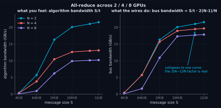
The left panel reports algbw and shows that larger groups are slower: 8 GPUs provide less than half the logical-tensor throughput of 2 GPUs. After applying the $2\frac{N-1}{N}$ traffic correction, the busbw curves in the right panel nearly overlap. The remaining difference, from 21.5 GB/s at $N{=}2$ to 17.8 GB/s at $N{=}8$, comes from topology: the 8-GPU ring crosses UPI, while the 2-GPU pair shares one PCIe switch. The derived traffic factor therefore explains most of the gap between the raw curves.
4.3 The latency floor: why small tensors are expensive
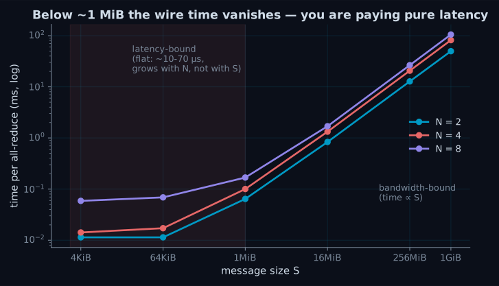
For $S \le 64$ KiB, the time curve is nearly flat. At $N{=}8$, a 4 KiB all-reduce and a 64 KiB all-reduce both take about 60–70 µs despite the 16× difference in bytes. The operation is dominated by the latency term $2(N-1)\alpha$. This latency floor rises from about 11 µs at $N{=}2$ to about 65 µs at $N{=}8$. Bandwidth begins to dominate at roughly 1 MiB on this machine.
A GPT-2 LayerNorm weight occupies only a few kilobytes. If a 124M model all-reduced each of its roughly 150 parameter tensors separately, the latency alone would be about $150 \times 65\,\mu\text{s} \approx 10$ ms per step. That is almost half the roughly 25 ms needed to synchronize the entire 250 MB bf16 model in one call, even though the small tensors contain only about 0.1% as many bytes. DDP avoids this overhead by grouping small gradients into larger buckets, the subject of the next post.
5. Reading along in real source
PyTorch DDP uses these same collective calls. It runs one all_reduce for each gradient bucket. The bucketing code is in torch/csrc/distributed/c10d/reducer.cpp and is called from torch.nn.parallel.DistributedDataParallel. ZeRO and FSDP instead use reduce_scatter_tensor and all_gather_into_tensor, as described in posts #3 and #4.
NCCL: channel construction is handled by the topology engine (ncclTopoCompute), while the two-phase pipelined ring is implemented in src/device/all_reduce.h. NCCL selects among ring and tree algorithms and the LL, LL128 and Simple protocols based on message size. The small change in the broadcast curve near 1 MiB in fig-4 reflects one such protocol transition.
MARS (our repository): the Moonlight-style optimizer in MARS (MARS/optimizers/muon.py) ends each step with dist.all_reduce(updates_flat). If $S$ is the total size of the parameters in bytes, this call makes each GPU send an additional $2\frac{N-1}{N}S$ bytes per step.
6. Summary
- Distributed training uses six basic collective primitives. All-reduce = reduce-scatter + all-gather, and our measurements confirm this identity within 3%.
- Ring all-reduce makes each GPU send $2\frac{N-1}{N}S < 2S$ bytes, so its per-GPU bandwidth volume remains bounded as $N$ grows. Its latency term, $2(N-1)\alpha$, still grows linearly with $N$ and dominates small-tensor collectives.
- Busbw enables fairer comparisons across primitives. The four ring-based collectives share the same bottleneck-link plateau, while rooted primitives approach one-way PCIe bandwidth, producing a 2.5× difference on the same machine.
- This machine’s numbers (pure PCIe, dual NUMA): ring collectives ~18 GB/s, point-to-point one-way ~50 GB/s, latency floor 11→65 µs (\(N\): 2→8), bandwidth/latency boundary ~1 MiB.
Next: Data Parallelism, part 1, from DP to DDP. Gradient synchronization sends $2\frac{N-1}{N}S$ bytes per GPU on every step. DDP reduces its visible cost by combining small gradients into buckets and overlapping communication with backward computation. The next post sweeps bucket_cap_mb from 1 to 500 to measure both effects.
Environment: 8× RTX PRO 6000 Blackwell, PyTorch 2.9.1, NCCL 2.27.5. Reproduce: torchrun --standalone --nproc_per_node={2,4,8} bench_collectives.py. Benchmark, plotting and schematic-generation code accompanies the series.
All benchmark scripts, schematic generators, plotting code and raw result CSVs for this post live in assets/blog/code/01-collective-communication.
Appendix: The Code That Ran
Every number in this post comes from the scripts below, embedded verbatim. Plotting and schematic code plus the raw result CSVs live in the folder linked above.
bench_collectives.py
"""
Collective communication primitive benchmark (Distributed Training Illustrated, post 01).

Benchmarks 6 primitives: broadcast / scatter / gather / all_gather / reduce_scatter / all_reduce
Conventions (matching the post):
  - S = logical message size (bytes of the full tensor)
  - algbw = S / t                          (algorithm bandwidth, the "user view")
  - busbw = algbw x correction factor      (bus bandwidth, the "hardware view", nccl-tests convention)
      all_reduce:      2(N-1)/N
      all_gather:      (N-1)/N
      reduce_scatter:  (N-1)/N
      broadcast:       1
      scatter/gather:  (N-1)/N

Usage:
  torchrun --standalone --nproc_per_node=8 bench_collectives.py --out ../results/collectives_n8.csv
"""

import argparse
import csv
import os

import torch
import torch.distributed as dist

SIZES = [4 * 2**10, 64 * 2**10, 2**20, 16 * 2**20, 256 * 2**20, 2**30]  # 4KiB..1GiB
DTYPE = torch.bfloat16


def bus_factor(op, n):
    return {
        "all_reduce": 2 * (n - 1) / n,
        "all_gather": (n - 1) / n,
        "reduce_scatter": (n - 1) / n,
        "broadcast": 1.0,
        "scatter": (n - 1) / n,
        "gather": (n - 1) / n,
    }[op]


def make_op(op, size_bytes, rank, world, device):
    """Return (fn, actually_allocated_ok). size_bytes is the logical message size S."""
    numel = size_bytes // DTYPE.itemsize
    # Ensure divisibility by world size (needed by scatter/gather/AG/RS)
    numel = (numel // world) * world
    if numel == 0:
        return None

    if op == "all_reduce":
        t = torch.randn(numel, dtype=DTYPE, device=device)
        return lambda: dist.all_reduce(t)

    if op == "broadcast":
        t = torch.randn(numel, dtype=DTYPE, device=device)
        return lambda: dist.broadcast(t, src=0)

    if op == "all_gather":
        out = torch.empty(numel, dtype=DTYPE, device=device)
        inp = torch.randn(numel // world, dtype=DTYPE, device=device)
        return lambda: dist.all_gather_into_tensor(out, inp)

    if op == "reduce_scatter":
        inp = torch.randn(numel, dtype=DTYPE, device=device)
        out = torch.empty(numel // world, dtype=DTYPE, device=device)
        return lambda: dist.reduce_scatter_tensor(out, inp)

    if op == "scatter":
        out = torch.empty(numel // world, dtype=DTYPE, device=device)
        if rank == 0:
            chunks = list(torch.randn(numel, dtype=DTYPE, device=device).chunk(world))
            return lambda: dist.scatter(out, chunks, src=0)
        return lambda: dist.scatter(out, None, src=0)

    if op == "gather":
        inp = torch.randn(numel // world, dtype=DTYPE, device=device)
        if rank == 0:
            outs = list(torch.empty(numel, dtype=DTYPE, device=device).chunk(world))
            return lambda: dist.gather(inp, outs, dst=0)
        return lambda: dist.gather(inp, None, dst=0)

    raise ValueError(op)


def bench(fn, iters, device):
    start = torch.cuda.Event(enable_timing=True)
    end = torch.cuda.Event(enable_timing=True)
    dist.barrier()
    torch.cuda.synchronize()
    start.record()
    for _ in range(iters):
        fn()
    end.record()
    torch.cuda.synchronize()
    return start.elapsed_time(end) / iters  # ms


def main():
    parser = argparse.ArgumentParser()
    parser.add_argument("--out", default="results.csv")
    args = parser.parse_args()

    rank = int(os.environ["RANK"])
    world = int(os.environ["WORLD_SIZE"])
    local_rank = int(os.environ["LOCAL_RANK"])
    torch.cuda.set_device(local_rank)
    device = torch.device("cuda", local_rank)
    dist.init_process_group("nccl", device_id=device)

    ops = ["broadcast", "scatter", "gather", "all_gather", "reduce_scatter", "all_reduce"]
    rows = []
    for op in ops:
        for size in SIZES:
            fn = make_op(op, size, rank, world, device)
            if fn is None:
                continue
            warmup = 20 if size < 256 * 2**20 else 5
            iters = 50 if size < 256 * 2**20 else 10
            for _ in range(warmup):
                fn()
            t_ms = bench(fn, iters, device)
            algbw = size / (t_ms / 1e3) / 1e9  # GB/s
            busbw = algbw * bus_factor(op, world)
            if rank == 0:
                rows.append([op, world, size, round(t_ms, 4), round(algbw, 2), round(busbw, 2)])
                print(f"{op:15s} N={world} S={size/2**20:9.3f}MiB  t={t_ms:9.3f}ms  algbw={algbw:7.2f}GB/s  busbw={busbw:7.2f}GB/s", flush=True)
            del fn
            torch.cuda.empty_cache()

    if rank == 0:
        os.makedirs(os.path.dirname(args.out) or ".", exist_ok=True)
        with open(args.out, "w", newline="") as f:
            w = csv.writer(f)
            w.writerow(["op", "world_size", "bytes", "time_ms", "algbw_GBps", "busbw_GBps"])
            w.writerows(rows)
        print(f"wrote {args.out}")

    dist.destroy_process_group()


if __name__ == "__main__":
    main()