Why A Single GPU Is Never Enough: A Map Of 5D Parallelism
A single GPU usually lacks both the memory and the compute needed to train a large model. This post explains those two limits through the 16Ψ memory ledger, then shows what each of the five parallelism dimensions splits. The rest of the series covers DP/DDP, ZeRO, FSDP, TP, SP/CP and PP one by one, with derivations, source-code references and experiments on an 8-GPU machine.
1. The two walls
Training a large model on one GPU runs into two limits: memory and time.
The memory limit. During training, each parameter is stored in several forms at the same time. Let $\Psi$ denote the number of parameters, so $\Psi = 7\times 10^9$ for a 7B model. With mixed precision and Adam, the memory ledger is:
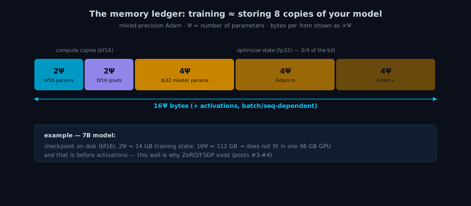
A useful rule of thumb is that training a model requires about eight times the memory needed to store its bf16 parameters. Three quarters of that total comes from fp32 master parameters and Adam states. Post #8 explains why model parameters can use bf16 while optimizer states remain in fp32, and post #3 shows how ZeRO shards this 12Ψ of replicated state. A 7B model needs 14 GB for its bf16 parameters but 112 GB for the full training state, which already exceeds our 96 GB GPUs. Activations require additional memory that grows with batch size and sequence length.
The time limit. Even if the model fits in memory, training requires roughly $6\Psi D$ FLOPs, where $D$ is the number of training tokens. The forward pass accounts for about $2\Psi D$ FLOPs and the backward pass for about $4\Psi D$. Training a 7B model on 1T tokens therefore requires $4.2\times 10^{22}$ FLOPs, or more than six years on one GPU at a realistic throughput of about 200 TFLOPS.
We therefore need multiple GPUs. Every multi-GPU training method must answer three questions:
What is split, which GPUs hold the resulting shards, and which collective operation combines them when needed?
2. Five dimensions, one map
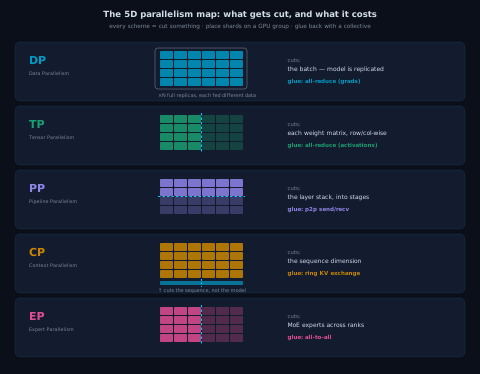
| Dimension | What it splits | Main limit addressed | Communication | Post |
|---|---|---|---|---|
| DP (data parallelism) | the batch (model replicated) | time (throughput) | all-reduce on gradients | #2 |
| TP (tensor parallelism) | each weight matrix, row/col-wise | memory (one layer too big) | all-reduce on activations | #5 |
| PP (pipeline parallelism) | the layer stack, into stages | memory (too many layers) | p2p send/recv | #7 |
| CP (context parallelism) | the sequence dimension | activation memory (long context) | ring KV exchange | #6 |
| EP (expert parallelism) | MoE experts | MoE parameter count | all-to-all | (season 2) |
Three related techniques do not define separate parallelism dimensions, but they are equally important:
- ZeRO / FSDP (posts #3 and #4) extend DP by sharding optimizer states, gradients and parameters across the DP group. Each layer still computes as a full replica, so these methods reduce storage, not computation.
- SP, sequence parallelism (post #6), is a companion to TP that shards the activations TP cannot reach (LayerNorm, dropout) along the sequence dimension.
- Mixed precision (post #8) explains why the ledger above uses both bf16 and fp32.
Large-scale training combines several of these dimensions. GPUs form a multidimensional grid, ep × pp × dp × cp × tp, and each GPU belongs to one communication group along every active dimension. The layout follows a practical rule: dimensions that communicate more often should use faster interconnects.
3. The common substrate: six collective primitives
Every entry in the table’s communication column uses the same six collective primitives: broadcast, scatter, gather, all-gather, reduce-scatter and all-reduce. These primitives provide a common unit for comparing methods throughout the series. DDP uses all-reduce for gradient synchronization, ZeRO uses reduce-scatter followed by all-gather, and FSDP prefetches parameters with pipelined all-gathers. To verify that one method communicates less than another, we first need to know the byte and time cost of each primitive.
Post #1 therefore begins with these primitives. It defines each operation, derives the $2\frac{N-1}{N}S$ communication volume of ring all-reduce, and measures bandwidth and latency on our 8-GPU machine. Normalizing the measurements by the derived traffic factors explains why different collectives produce different raw bandwidth curves.
4. Series roadmap
- Collective communication primitives: how the all-reduce bill is computed ✅
- Data parallelism, part 1: from DP to DDP, with bucketing and compute/comm overlap
- Data parallelism, part 2: ZeRO’s three-stage ledger of zero redundancy
- FSDP: how PyTorch implements ZeRO-3 (FSDP1 vs FSDP2)
- Tensor parallelism: Megatron’s two cuts
- Sequence & context parallelism: two ways to cut the sequence
- Pipeline parallelism: the geometry of bubbles
- Mixed precision: the numerics ledger of the bf16 era
- Optimizers in a sharded world: why row-local operators work well with distributed sharding
All experiments run on one machine with 8× RTX PRO 6000 Blackwell GPUs (96 GB), PCIe without NVLink, PyTorch 2.9.1 and NCCL 2.27.5. Because the machine has no NVLink, communication bottlenecks are easier to observe.
References: the HuggingFace Ultra-Scale Playbook, the nanotron, Megatron-LM and DeepSpeed source trees, and the 图解大模型训练 series by 猛猿. All schematics and plots in this series are original, generated by code published alongside each post.
Schematic-generation code for this post lives in assets/blog/code/00-series-overview.